General Hamiltonians#
This notebook shows how to build and encode Fermionic Hamiltonians with ferrmion. You can easily define any Hamiltonian you like, and there are some functions to make it even easier to create common Hamiltonians. If you want to see that, skip to the next section.
The encodings used in this notebook are known as the naive versions of each encoding, because there is almost definitely a better version of it. ferrmion provides methods to get encodings optimised for your Hamiltonian. Check those out in the Optimized Encodings notebook.
If you need to go a step further and define your own encoding to optimise, you can do that too! Start with the Ternary Tree Mappings notebook.
Defining a Hamiltonian#
Fermionic hamiltonians are built up of a number of terms, each of which has:
a “signature” of fermionic ladder opertors “+” and “-”
a matrix of coefficients
You can build up arbitrary Hamiltonians by creating an empty one and adding terms.
Let’s create one with a “+-” or onsite term for a system with 5 fermionic modes (orbitals or sites!).
import ferrmion as fr
import numpy as np

fham = fr.FermionHamiltonian()
n_modes = 5
onsite_coefficients = np.random.random(tuple([n_modes]*2))
fham.add_constant(10.0)
fham.creation().annihilation().with_coefficients(onsite_coefficients)
FermionHamiltonian(+-, 5 modes, constant 10)
we could add an interaction term “+-+-” in the same way, making sure to keep the number of modes constant.
interaction_coefficients = np.random.random(tuple([n_modes]*4))

fham.creation().annihilation().creation().annihilation().with_coefficients(
    interaction_coefficients
)
FermionHamiltonian(+-, +-+-, 5 modes, constant 10)
Encoding a Hamiltonian.#
To encode a FermionHamiltonian into a QubitHamiltonian, we can either build an encoding using the TernaryTree class, or use an inbuilt encoding. Building your gives you lots more flexability but if you just want to encode a Hamiltonian, you can still use the optimisation methods in ferrmion if you like.
By default, ferrmion optimises TernaryTree encodings for you, but you can also use the naive (unoptimised) versions of the encodings.
fr.JordanWigner(n_modes).encode(fham)
QubitHamiltonian({'IIIII': 18.9076311490779+0i, 'IIIIZ': -1.8455210285622243+0i, 'IIIXX': 1.5570252447720878+0i, 'IIIXY': 0-0.054044855267008036i, 'IIIYX': 0+0.05404485526700803i, 'IIIYY': 1.5570252447720878+0i, 'IIIZI': -1.904902251450257+0i, 'IIIZZ': 0.0673032609026337+0i, 'IIXIX': -0.052942896570146475+0i, 'IIXIY': 0-0.06155836006233255i, 'IIXXI': 0.9821509553048453+0i, 'IIXXZ': -0.028728638861985636+0i, 'IIXYI': 0-0.1852474642087414i, 'IIXYZ': 0+0.11200173928332946i, 'IIXZX': 1.9185776348309769+0i, 'IIXZY': 0+0.2886439877855828i, 'IIYIX': 0+0.06155836006233255i, 'IIYIY': -0.052942896570146475+0i, 'IIYXI': 0+0.1852474642087414i, 'IIYXZ': 0-0.11200173928332946i, 'IIYYI': 0.9821509553048453+0i, 'IIYYZ': -0.028728638861985636+0i, 'IIYZX': 0-0.2886439877855828i, 'IIYZY': 1.9185776348309769+0i, 'IIZII': -1.72887707489718+0i, 'IIZIZ': 0.17882256940610555+0i, 'IIZXX': -0.013420657293724284+0i, 'IIZXY': 0+0.08955283111864738i, 'IIZYX': 0-0.08955283111864738i, 'IIZYY': -0.013420657293724284+0i, 'IIZZI': -0.27698557118510925+0i, 'IXIXI': 0.0964500346445237+0i, 'IXIYI': 0+0.06285586618432534i, 'IXIZX': -0.06423161271570207+0i, 'IXIZY': 0+0.025195599696344426i, 'IXXII': 1.1994994625822795+0i, 'IXXIZ': -0.04923414895740931+0i, 'IXXXX': -0.09925610140318297+0i, 'IXXXY': 0+0.07648708675243585i, 'IXXYX': 0-0.1261284629092859i, 'IXXYY': 0.0010532232694588708+0i, 'IXXZI': -0.08678963265897728+0i, 'IXYII': 0+0.09194528485148387i, 'IXYIZ': 0+0.028231230883319566i, 'IXYXX': 0-0.049921846765950344i, 'IXYXY': -0.09372480058823673+0i, 'IXYYX': -0.006584524084405144+0i, 'IXYYY': 0-0.09956322292280037i, 'IXYZI': 0-0.06398062582554465i, 'IXZIX': 0.0023960952626263035+0i, 'IXZIY': 0+0.06343039093935693i, 'IXZXI': 1.5426745194253009+0i, 'IXZXZ': -0.2608224533564394+0i, 'IXZYI': 0-0.0014603929204522331i, 'IXZYZ': 0+0.10604779756515971i, 'IXZZX': 1.8448827340725749+0i, 'IXZZY': 0+0.11979992248556479i, 'IYIXI': 0-0.06285586618432534i, 'IYIYI': 0.0964500346445237+0i, 'IYIZX': 0-0.025195599696344426i, 'IYIZY': -0.06423161271570207+0i, 'IYXII': 0-0.09194528485148387i, 'IYXIZ': 0-0.028231230883319566i, 'IYXXX': 0+0.09956322292280037i, 'IYXXY': -0.006584524084405144+0i, 'IYXYX': -0.09372480058823673+0i, 'IYXYY': 0+0.049921846765950344i, 'IYXZI': 0+0.06398062582554465i, 'IYYII': 1.1994994625822795+0i, 'IYYIZ': -0.04923414895740931+0i, 'IYYXX': 0.0010532232694588708+0i, 'IYYXY': 0+0.1261284629092859i, 'IYYYX': 0-0.07648708675243585i, 'IYYYY': -0.09925610140318297+0i, 'IYYZI': -0.08678963265897728+0i, 'IYZIX': 0-0.06343039093935693i, 'IYZIY': 0.0023960952626263035+0i, 'IYZXI': 0+0.0014603929204522192i, 'IYZXZ': 0-0.10604779756515971i, 'IYZYI': 1.542674519425301+0i, 'IYZYZ': -0.2608224533564394+0i, 'IYZZX': 0-0.11979992248556484i, 'IYZZY': 1.8448827340725749+0i, 'IZIII': -1.68467299764772+0i, 'IZIIZ': -0.15210632381365122+0i, 'IZIXX': -0.010695135161692848+0i, 'IZIXY': 0+0.19156313631216412i, 'IZIYX': 0-0.19156313631216412i, 'IZIYY': -0.010695135161692848+0i, 'IZIZI': 0.12094142501269206+0i, 'IZXXI': 0.0028929733946117947+0i, 'IZXYI': 0-0.000371862414990376i, 'IZXZX': 0.06284428800744621+0i, 'IZXZY': 0-0.0056239564519726115i, 'IZYXI': 0+0.000371862414990376i, 'IZYYI': 0.0028929733946117947+0i, 'IZYZX': 0+0.0056239564519726115i, 'IZYZY': 0.06284428800744621+0i, 'IZZII': -0.11297254852969835+0i, 'XIXII': -0.047969782988100604+0i, 'XIYII': 0-0.029077434415576822i, 'XIZXI': 0.1138254471881604+0i, 'XIZYI': 0-0.004000859283264102i, 'XIZZX': -0.03297255049414944+0i, 'XIZZY': 0+0.1309089557676221i, 'XXIII': 1.582247638867951+0i, 'XXIIZ': 0.18967756459337848+0i, 'XXIXX': 0.003345975475951654+0i, 'XXIXY': 0+0.04930293648353505i, 'XXIYX': 0-0.09495336844411444i, 'XXIYY': -0.08236776193900117+0i, 'XXIZI': -0.1717432403988048+0i, 'XXXXI': 0.08616243879189722+0i, 'XXXYI': 0-0.11047588353539639i, 'XXXZX': -0.15431958544598434+0i, 'XXXZY': 0+0.050613718300248814i, 'XXYXI': 0+0.1147865789519015i, 'XXYYI': 0.09669961196484247+0i, 'XXYZX': 0-0.0013451335457962538i, 'XXYZY': 0.017578033928802375+0i, 'XXZII': 0.0785806254379065+0i, 'XYIII': 0-0.07787606730090726i, 'XYIIZ': 0-0.09109713050673937i, 'XYIXX': 0+0.14183929138880882i, 'XYIXY': 0.07143231291895069+0i, 'XYIYX': 0.01428142449600213+0i, 'XYIYY': 0+0.09618885942822944i, 'XYIZI': 0+0.053815241763404714i, 'XYXXI': 0+0.06824766115154023i, 'XYXYI': -0.0743562581682904+0i, 'XYXZX': 0+0.026941749471265278i, 'XYXZY': -0.20180847815216735+0i, 'XYYXI': 0.06381908499534518+0i, 'XYYYI': 0+0.07255835656804532i, 'XYYZX': 0.029910858777380596+0i, 'XYYZY': 0+0.07621033422571782i, 'XYZII': 0-0.14753041107216724i, 'XZIXI': -0.013534287040473186+0i, 'XZIYI': 0+0.047632417724760207i, 'XZIZX': 0.10890704797913282+0i, 'XZIZY': 0-0.12409578016633006i, 'XZXII': 1.4711723106655499+0i, 'XZXIZ': -0.06045787993999069+0i, 'XZXXX': -0.07219065566469819+0i, 'XZXXY': 0+0.11483104614317448i, 'XZXYX': 0-0.1156359828044034i, 'XZXYY': -0.08139498712268023+0i, 'XZXZI': 0.00006576012327344505+0i, 'XZYII': 0-0.034269571238060716i, 'XZYIZ': 0-0.15167760447941508i, 'XZYXX': 0-0.00658192394259384i, 'XZYXY': 0.055614191102423896+0i, 'XZYYX': -0.046409859644441845+0i, 'XZYYY': 0-0.007386860603822737i, 'XZYZI': 0+0.006233734843999736i, 'XZZIX': -0.011860886922600886+0i, 'XZZIY': 0-0.1503265878280932i, 'XZZXI': 1.6506869653492973+0i, 'XZZXZ': 0.016650803881969836+0i, 'XZZYI': 0+0.12203034124991721i, 'XZZYZ': 0-0.024813275586719835i, 'XZZZX': 1.360399359433127+0i, 'XZZZY': 0+0.05083052297699031i, 'YIXII': 0+0.029077434415576822i, 'YIYII': -0.047969782988100604+0i, 'YIZXI': 0+0.004000859283264102i, 'YIZYI': 0.1138254471881604+0i, 'YIZZX': 0-0.1309089557676221i, 'YIZZY': -0.03297255049414944+0i, 'YXIII': 0+0.07787606730090726i, 'YXIIZ': 0+0.09109713050673937i, 'YXIXX': 0-0.09618885942822944i, 'YXIXY': 0.01428142449600213+0i, 'YXIYX': 0.07143231291895069+0i, 'YXIYY': 0-0.14183929138880882i, 'YXIZI': 0-0.053815241763404714i, 'YXXXI': 0-0.07255835656804532i, 'YXXYI': 0.06381908499534518+0i, 'YXXZX': 0-0.07621033422571782i, 'YXXZY': 0.029910858777380596+0i, 'YXYXI': -0.0743562581682904+0i, 'YXYYI': 0-0.06824766115154023i, 'YXYZX': -0.20180847815216735+0i, 'YXYZY': 0-0.026941749471265278i, 'YXZII': 0+0.14753041107216724i, 'YYIII': 1.582247638867951+0i, 'YYIIZ': 0.18967756459337848+0i, 'YYIXX': -0.08236776193900117+0i, 'YYIXY': 0+0.09495336844411444i, 'YYIYX': 0-0.04930293648353505i, 'YYIYY': 0.003345975475951654+0i, 'YYIZI': -0.1717432403988048+0i, 'YYXXI': 0.09669961196484247+0i, 'YYXYI': 0-0.1147865789519015i, 'YYXZX': 0.017578033928802375+0i, 'YYXZY': 0+0.0013451335457962538i, 'YYYXI': 0+0.11047588353539639i, 'YYYYI': 0.08616243879189722+0i, 'YYYZX': 0-0.050613718300248814i, 'YYYZY': -0.15431958544598434+0i, 'YYZII': 0.0785806254379065+0i, 'YZIXI': 0-0.047632417724760207i, 'YZIYI': -0.013534287040473186+0i, 'YZIZX': 0+0.12409578016633006i, 'YZIZY': 0.10890704797913282+0i, 'YZXII': 0+0.034269571238060716i, 'YZXIZ': 0+0.15167760447941508i, 'YZXXX': 0+0.007386860603822737i, 'YZXXY': -0.046409859644441845+0i, 'YZXYX': 0.055614191102423896+0i, 'YZXYY': 0+0.00658192394259384i, 'YZXZI': 0-0.006233734843999736i, 'YZYII': 1.4711723106655497+0i, 'YZYIZ': -0.06045787993999069+0i, 'YZYXX': -0.08139498712268023+0i, 'YZYXY': 0+0.1156359828044034i, 'YZYYX': 0-0.11483104614317448i, 'YZYYY': -0.07219065566469819+0i, 'YZYZI': 0.00006576012327344505+0i, 'YZZIX': 0+0.1503265878280932i, 'YZZIY': -0.011860886922600886+0i, 'YZZXI': 0-0.12203034124991721i, 'YZZXZ': 0+0.024813275586719835i, 'YZZYI': 1.6506869653492973+0i, 'YZZYZ': 0.016650803881969836+0i, 'YZZZX': 0-0.05083052297699031i, 'YZZZY': 1.3603993594331272+0i, 'ZIIII': -2.0188019671438022+0i, 'ZIIIZ': -0.08859828295605188+0i, 'ZIIXX': 0.036287664861934577+0i, 'ZIIXY': 0-0.11771942960799285i, 'ZIIYX': 0+0.11771942960799285i, 'ZIIYY': 0.036287664861934577+0i, 'ZIIZI': 0.13048181384245677+0i, 'ZIXXI': 0.21512383704203647+0i, 'ZIXYI': 0+0.0565412987386498i, 'ZIXZX': -0.2322946066416891+0i, 'ZIXZY': 0+0.029093525733964468i, 'ZIYXI': 0-0.0565412987386498i, 'ZIYYI': 0.21512383704203647+0i, 'ZIYZX': 0-0.029093525733964468i, 'ZIYZY': -0.2322946066416891+0i, 'ZIZII': 0.17251072768185632+0i, 'ZXXII': 0.03699300251288758+0i, 'ZXYII': 0-0.14908376856335048i, 'ZXZXI': 0.09638481832588006+0i, 'ZXZYI': 0-0.01060990101616291i, 'ZXZZX': -0.09951450710339771+0i, 'ZXZZY': 0-0.27078507170064003i, 'ZYXII': 0+0.14908376856335048i, 'ZYYII': 0.03699300251288758+0i, 'ZYZXI': 0+0.01060990101616291i, 'ZYZYI': 0.09638481832588006+0i, 'ZYZZX': 0+0.27078507170064003i, 'ZYZZY': -0.09951450710339771+0i, 'ZZIII': 0.23574710026205084+0i})
fr.JordanWigner(n_modes).encode_naive(fham)
QubitHamiltonian({'IIIII': 18.9076311490779+0i, 'IIIIZ': -1.8455210285622243+0i, 'IIIXX': 1.5570252447720878+0i, 'IIIXY': 0-0.054044855267008036i, 'IIIYX': 0+0.05404485526700803i, 'IIIYY': 1.5570252447720878+0i, 'IIIZI': -1.904902251450257+0i, 'IIIZZ': 0.0673032609026337+0i, 'IIXIX': -0.052942896570146475+0i, 'IIXIY': 0-0.06155836006233255i, 'IIXXI': 0.9821509553048453+0i, 'IIXXZ': -0.028728638861985636+0i, 'IIXYI': 0-0.1852474642087414i, 'IIXYZ': 0+0.11200173928332946i, 'IIXZX': 1.9185776348309769+0i, 'IIXZY': 0+0.2886439877855828i, 'IIYIX': 0+0.06155836006233255i, 'IIYIY': -0.052942896570146475+0i, 'IIYXI': 0+0.1852474642087414i, 'IIYXZ': 0-0.11200173928332946i, 'IIYYI': 0.9821509553048453+0i, 'IIYYZ': -0.028728638861985636+0i, 'IIYZX': 0-0.2886439877855828i, 'IIYZY': 1.9185776348309769+0i, 'IIZII': -1.72887707489718+0i, 'IIZIZ': 0.17882256940610555+0i, 'IIZXX': -0.013420657293724284+0i, 'IIZXY': 0+0.08955283111864738i, 'IIZYX': 0-0.08955283111864738i, 'IIZYY': -0.013420657293724284+0i, 'IIZZI': -0.27698557118510925+0i, 'IXIXI': 0.0964500346445237+0i, 'IXIYI': 0+0.06285586618432534i, 'IXIZX': -0.06423161271570207+0i, 'IXIZY': 0+0.025195599696344426i, 'IXXII': 1.1994994625822795+0i, 'IXXIZ': -0.04923414895740931+0i, 'IXXXX': -0.09925610140318297+0i, 'IXXXY': 0+0.07648708675243585i, 'IXXYX': 0-0.1261284629092859i, 'IXXYY': 0.0010532232694588708+0i, 'IXXZI': -0.08678963265897728+0i, 'IXYII': 0+0.09194528485148387i, 'IXYIZ': 0+0.028231230883319566i, 'IXYXX': 0-0.049921846765950344i, 'IXYXY': -0.09372480058823673+0i, 'IXYYX': -0.006584524084405144+0i, 'IXYYY': 0-0.09956322292280037i, 'IXYZI': 0-0.06398062582554465i, 'IXZIX': 0.0023960952626263035+0i, 'IXZIY': 0+0.06343039093935693i, 'IXZXI': 1.5426745194253009+0i, 'IXZXZ': -0.2608224533564394+0i, 'IXZYI': 0-0.0014603929204522331i, 'IXZYZ': 0+0.10604779756515971i, 'IXZZX': 1.8448827340725749+0i, 'IXZZY': 0+0.11979992248556479i, 'IYIXI': 0-0.06285586618432534i, 'IYIYI': 0.0964500346445237+0i, 'IYIZX': 0-0.025195599696344426i, 'IYIZY': -0.06423161271570207+0i, 'IYXII': 0-0.09194528485148387i, 'IYXIZ': 0-0.028231230883319566i, 'IYXXX': 0+0.09956322292280037i, 'IYXXY': -0.006584524084405144+0i, 'IYXYX': -0.09372480058823673+0i, 'IYXYY': 0+0.049921846765950344i, 'IYXZI': 0+0.06398062582554465i, 'IYYII': 1.1994994625822795+0i, 'IYYIZ': -0.04923414895740931+0i, 'IYYXX': 0.0010532232694588708+0i, 'IYYXY': 0+0.1261284629092859i, 'IYYYX': 0-0.07648708675243585i, 'IYYYY': -0.09925610140318297+0i, 'IYYZI': -0.08678963265897728+0i, 'IYZIX': 0-0.06343039093935693i, 'IYZIY': 0.0023960952626263035+0i, 'IYZXI': 0+0.0014603929204522192i, 'IYZXZ': 0-0.10604779756515971i, 'IYZYI': 1.542674519425301+0i, 'IYZYZ': -0.2608224533564394+0i, 'IYZZX': 0-0.11979992248556484i, 'IYZZY': 1.8448827340725749+0i, 'IZIII': -1.68467299764772+0i, 'IZIIZ': -0.15210632381365122+0i, 'IZIXX': -0.010695135161692848+0i, 'IZIXY': 0+0.19156313631216412i, 'IZIYX': 0-0.19156313631216412i, 'IZIYY': -0.010695135161692848+0i, 'IZIZI': 0.12094142501269206+0i, 'IZXXI': 0.0028929733946117947+0i, 'IZXYI': 0-0.000371862414990376i, 'IZXZX': 0.06284428800744621+0i, 'IZXZY': 0-0.0056239564519726115i, 'IZYXI': 0+0.000371862414990376i, 'IZYYI': 0.0028929733946117947+0i, 'IZYZX': 0+0.0056239564519726115i, 'IZYZY': 0.06284428800744621+0i, 'IZZII': -0.11297254852969835+0i, 'XIXII': -0.047969782988100604+0i, 'XIYII': 0-0.029077434415576822i, 'XIZXI': 0.1138254471881604+0i, 'XIZYI': 0-0.004000859283264102i, 'XIZZX': -0.03297255049414944+0i, 'XIZZY': 0+0.1309089557676221i, 'XXIII': 1.582247638867951+0i, 'XXIIZ': 0.18967756459337848+0i, 'XXIXX': 0.003345975475951654+0i, 'XXIXY': 0+0.04930293648353505i, 'XXIYX': 0-0.09495336844411444i, 'XXIYY': -0.08236776193900117+0i, 'XXIZI': -0.1717432403988048+0i, 'XXXXI': 0.08616243879189722+0i, 'XXXYI': 0-0.11047588353539639i, 'XXXZX': -0.15431958544598434+0i, 'XXXZY': 0+0.050613718300248814i, 'XXYXI': 0+0.1147865789519015i, 'XXYYI': 0.09669961196484247+0i, 'XXYZX': 0-0.0013451335457962538i, 'XXYZY': 0.017578033928802375+0i, 'XXZII': 0.0785806254379065+0i, 'XYIII': 0-0.07787606730090726i, 'XYIIZ': 0-0.09109713050673937i, 'XYIXX': 0+0.14183929138880882i, 'XYIXY': 0.07143231291895069+0i, 'XYIYX': 0.01428142449600213+0i, 'XYIYY': 0+0.09618885942822944i, 'XYIZI': 0+0.053815241763404714i, 'XYXXI': 0+0.06824766115154023i, 'XYXYI': -0.0743562581682904+0i, 'XYXZX': 0+0.026941749471265278i, 'XYXZY': -0.20180847815216735+0i, 'XYYXI': 0.06381908499534518+0i, 'XYYYI': 0+0.07255835656804532i, 'XYYZX': 0.029910858777380596+0i, 'XYYZY': 0+0.07621033422571782i, 'XYZII': 0-0.14753041107216724i, 'XZIXI': -0.013534287040473186+0i, 'XZIYI': 0+0.047632417724760207i, 'XZIZX': 0.10890704797913282+0i, 'XZIZY': 0-0.12409578016633006i, 'XZXII': 1.4711723106655499+0i, 'XZXIZ': -0.06045787993999069+0i, 'XZXXX': -0.07219065566469819+0i, 'XZXXY': 0+0.11483104614317448i, 'XZXYX': 0-0.1156359828044034i, 'XZXYY': -0.08139498712268023+0i, 'XZXZI': 0.00006576012327344505+0i, 'XZYII': 0-0.034269571238060716i, 'XZYIZ': 0-0.15167760447941508i, 'XZYXX': 0-0.00658192394259384i, 'XZYXY': 0.055614191102423896+0i, 'XZYYX': -0.046409859644441845+0i, 'XZYYY': 0-0.007386860603822737i, 'XZYZI': 0+0.006233734843999736i, 'XZZIX': -0.011860886922600886+0i, 'XZZIY': 0-0.1503265878280932i, 'XZZXI': 1.6506869653492973+0i, 'XZZXZ': 0.016650803881969836+0i, 'XZZYI': 0+0.12203034124991721i, 'XZZYZ': 0-0.024813275586719835i, 'XZZZX': 1.360399359433127+0i, 'XZZZY': 0+0.05083052297699031i, 'YIXII': 0+0.029077434415576822i, 'YIYII': -0.047969782988100604+0i, 'YIZXI': 0+0.004000859283264102i, 'YIZYI': 0.1138254471881604+0i, 'YIZZX': 0-0.1309089557676221i, 'YIZZY': -0.03297255049414944+0i, 'YXIII': 0+0.07787606730090726i, 'YXIIZ': 0+0.09109713050673937i, 'YXIXX': 0-0.09618885942822944i, 'YXIXY': 0.01428142449600213+0i, 'YXIYX': 0.07143231291895069+0i, 'YXIYY': 0-0.14183929138880882i, 'YXIZI': 0-0.053815241763404714i, 'YXXXI': 0-0.07255835656804532i, 'YXXYI': 0.06381908499534518+0i, 'YXXZX': 0-0.07621033422571782i, 'YXXZY': 0.029910858777380596+0i, 'YXYXI': -0.0743562581682904+0i, 'YXYYI': 0-0.06824766115154023i, 'YXYZX': -0.20180847815216735+0i, 'YXYZY': 0-0.026941749471265278i, 'YXZII': 0+0.14753041107216724i, 'YYIII': 1.582247638867951+0i, 'YYIIZ': 0.18967756459337848+0i, 'YYIXX': -0.08236776193900117+0i, 'YYIXY': 0+0.09495336844411444i, 'YYIYX': 0-0.04930293648353505i, 'YYIYY': 0.003345975475951654+0i, 'YYIZI': -0.1717432403988048+0i, 'YYXXI': 0.09669961196484247+0i, 'YYXYI': 0-0.1147865789519015i, 'YYXZX': 0.017578033928802375+0i, 'YYXZY': 0+0.0013451335457962538i, 'YYYXI': 0+0.11047588353539639i, 'YYYYI': 0.08616243879189722+0i, 'YYYZX': 0-0.050613718300248814i, 'YYYZY': -0.15431958544598434+0i, 'YYZII': 0.0785806254379065+0i, 'YZIXI': 0-0.047632417724760207i, 'YZIYI': -0.013534287040473186+0i, 'YZIZX': 0+0.12409578016633006i, 'YZIZY': 0.10890704797913282+0i, 'YZXII': 0+0.034269571238060716i, 'YZXIZ': 0+0.15167760447941508i, 'YZXXX': 0+0.007386860603822737i, 'YZXXY': -0.046409859644441845+0i, 'YZXYX': 0.055614191102423896+0i, 'YZXYY': 0+0.00658192394259384i, 'YZXZI': 0-0.006233734843999736i, 'YZYII': 1.4711723106655497+0i, 'YZYIZ': -0.06045787993999069+0i, 'YZYXX': -0.08139498712268023+0i, 'YZYXY': 0+0.1156359828044034i, 'YZYYX': 0-0.11483104614317448i, 'YZYYY': -0.07219065566469819+0i, 'YZYZI': 0.00006576012327344505+0i, 'YZZIX': 0+0.1503265878280932i, 'YZZIY': -0.011860886922600886+0i, 'YZZXI': 0-0.12203034124991721i, 'YZZXZ': 0+0.024813275586719835i, 'YZZYI': 1.6506869653492973+0i, 'YZZYZ': 0.016650803881969836+0i, 'YZZZX': 0-0.05083052297699031i, 'YZZZY': 1.3603993594331272+0i, 'ZIIII': -2.0188019671438022+0i, 'ZIIIZ': -0.08859828295605188+0i, 'ZIIXX': 0.036287664861934577+0i, 'ZIIXY': 0-0.11771942960799285i, 'ZIIYX': 0+0.11771942960799285i, 'ZIIYY': 0.036287664861934577+0i, 'ZIIZI': 0.13048181384245677+0i, 'ZIXXI': 0.21512383704203647+0i, 'ZIXYI': 0+0.0565412987386498i, 'ZIXZX': -0.2322946066416891+0i, 'ZIXZY': 0+0.029093525733964468i, 'ZIYXI': 0-0.0565412987386498i, 'ZIYYI': 0.21512383704203647+0i, 'ZIYZX': 0-0.029093525733964468i, 'ZIYZY': -0.2322946066416891+0i, 'ZIZII': 0.17251072768185632+0i, 'ZXXII': 0.03699300251288758+0i, 'ZXYII': 0-0.14908376856335048i, 'ZXZXI': 0.09638481832588006+0i, 'ZXZYI': 0-0.01060990101616291i, 'ZXZZX': -0.09951450710339771+0i, 'ZXZZY': 0-0.27078507170064003i, 'ZYXII': 0+0.14908376856335048i, 'ZYYII': 0.03699300251288758+0i, 'ZYZXI': 0+0.01060990101616291i, 'ZYZYI': 0.09638481832588006+0i, 'ZYZZX': 0+0.27078507170064003i, 'ZYZZY': -0.09951450710339771+0i, 'ZZIII': 0.23574710026205084+0i})
fr.JordanWigner(n_modes).encode_annealed(fham)
QubitHamiltonian({'IIIII': 18.9076311490779+0i, 'IIIIZ': -1.904902251450257+0i, 'IIIXX': 1.6506869653492973+0i, 'IIIXY': 0+0.12203034124991721i, 'IIIYX': 0-0.12203034124991721i, 'IIIYY': 1.6506869653492973+0i, 'IIIZI': -2.0188019671438022+0i, 'IIIZZ': 0.13048181384245677+0i, 'IIXIX': 0.21512383704203647+0i, 'IIXIY': 0+0.0565412987386498i, 'IIXXI': 1.4711723106655497+0i, 'IIXXZ': 0.00006576012327344505+0i, 'IIXYI': 0+0.034269571238060716i, 'IIXYZ': 0-0.006233734843999736i, 'IIXZX': 0.9821509553048453+0i, 'IIXZY': 0-0.1852474642087414i, 'IIYIX': 0-0.0565412987386498i, 'IIYIY': 0.21512383704203647+0i, 'IIYXI': 0-0.034269571238060716i, 'IIYXZ': 0+0.006233734843999736i, 'IIYYI': 1.4711723106655499+0i, 'IIYYZ': 0.00006576012327344505+0i, 'IIYZX': 0+0.1852474642087414i, 'IIYZY': 0.9821509553048453+0i, 'IIZII': -1.72887707489718+0i, 'IIZIZ': -0.27698557118510925+0i, 'IIZXX': -0.013534287040473186+0i, 'IIZXY': 0+0.047632417724760207i, 'IIZYX': 0-0.047632417724760207i, 'IIZYY': -0.013534287040473186+0i, 'IIZZI': 0.17251072768185632+0i, 'IXIXI': 0.0785806254379065+0i, 'IXIYI': 0+0.14753041107216724i, 'IXIZX': 0.0964500346445237+0i, 'IXIZY': 0+0.06285586618432534i, 'IXXII': 1.1994994625822795+0i, 'IXXIZ': -0.08678963265897728+0i, 'IXXXX': -0.06381908499534518+0i, 'IXXXY': 0-0.07255835656804532i, 'IXXYX': 0-0.11047588353539639i, 'IXXYY': -0.08616243879189722+0i, 'IXXZI': 0.03699300251288758+0i, 'IXYII': 0+0.09194528485148387i, 'IXYIZ': 0-0.06398062582554465i, 'IXYXX': 0+0.06824766115154023i, 'IXYXY': -0.0743562581682904+0i, 'IXYYX': 0.09669961196484247+0i, 'IXYYY': 0-0.1147865789519015i, 'IXYZI': 0-0.14908376856335048i, 'IXZIX': 0.09638481832588006+0i, 'IXZIY': 0-0.01060990101616291i, 'IXZXI': 1.582247638867951+0i, 'IXZXZ': -0.1717432403988048+0i, 'IXZYI': 0+0.07787606730090726i, 'IXZYZ': 0-0.053815241763404714i, 'IXZZX': 1.5426745194253009+0i, 'IXZZY': 0-0.0014603929204522331i, 'IYIXI': 0-0.14753041107216724i, 'IYIYI': 0.0785806254379065+0i, 'IYIZX': 0-0.06285586618432534i, 'IYIZY': 0.0964500346445237+0i, 'IYXII': 0-0.09194528485148387i, 'IYXIZ': 0+0.06398062582554465i, 'IYXXX': 0+0.1147865789519015i, 'IYXXY': 0.09669961196484247+0i, 'IYXYX': -0.0743562581682904+0i, 'IYXYY': 0-0.06824766115154023i, 'IYXZI': 0+0.14908376856335048i, 'IYYII': 1.1994994625822795+0i, 'IYYIZ': -0.08678963265897728+0i, 'IYYXX': -0.08616243879189722+0i, 'IYYXY': 0+0.11047588353539639i, 'IYYYX': 0+0.07255835656804532i, 'IYYYY': -0.06381908499534518+0i, 'IYYZI': 0.03699300251288758+0i, 'IYZIX': 0+0.01060990101616291i, 'IYZIY': 0.09638481832588006+0i, 'IYZXI': 0-0.07787606730090726i, 'IYZXZ': 0+0.053815241763404714i, 'IYZYI': 1.582247638867951+0i, 'IYZYZ': -0.1717432403988048+0i, 'IYZZX': 0+0.0014603929204522192i, 'IYZZY': 1.542674519425301+0i, 'IZIII': -1.68467299764772+0i, 'IZIIZ': 0.12094142501269206+0i, 'IZIXX': 0.1138254471881604+0i, 'IZIXY': 0-0.004000859283264102i, 'IZIYX': 0+0.004000859283264102i, 'IZIYY': 0.1138254471881604+0i, 'IZIZI': 0.23574710026205084+0i, 'IZXXI': -0.047969782988100604+0i, 'IZXYI': 0+0.029077434415576822i, 'IZXZX': 0.0028929733946117947+0i, 'IZXZY': 0-0.000371862414990376i, 'IZYXI': 0-0.029077434415576822i, 'IZYYI': -0.047969782988100604+0i, 'IZYZX': 0+0.000371862414990376i, 'IZYZY': 0.0028929733946117947+0i, 'IZZII': -0.11297254852969835+0i, 'XIXII': 0.06284428800744621+0i, 'XIYII': 0+0.0056239564519726115i, 'XIZXI': -0.03297255049414944+0i, 'XIZYI': 0-0.1309089557676221i, 'XIZZX': -0.010695135161692848+0i, 'XIZZY': 0-0.19156313631216412i, 'XXIII': 1.8448827340725749+0i, 'XXIIZ': 0.0023960952626263035+0i, 'XXIXX': 0.08236776193900117+0i, 'XXIXY': 0+0.04930293648353505i, 'XXIYX': 0+0.14183929138880882i, 'XXIYY': 0.01428142449600213+0i, 'XXIZI': -0.09951450710339771+0i, 'XXXXI': 0.029910858777380596+0i, 'XXXYI': 0-0.050613718300248814i, 'XXXZX': 0.09925610140318297+0i, 'XXXZY': 0+0.1261284629092859i, 'XXYXI': 0-0.026941749471265278i, 'XXYYI': -0.017578033928802375+0i, 'XXYZX': 0+0.049921846765950344i, 'XXYZY': 0.006584524084405144+0i, 'XXZII': -0.06423161271570207+0i, 'XYIII': 0-0.11979992248556479i, 'XYIIZ': 0-0.06343039093935693i, 'XYIXX': 0-0.09618885942822944i, 'XYIXY': 0.07143231291895069+0i, 'XYIYX': -0.003345975475951654+0i, 'XYIYY': 0+0.09495336844411444i, 'XYIZI': 0+0.27078507170064003i, 'XYXXI': 0+0.0013451335457962538i, 'XYXYI': 0.20180847815216735+0i, 'XYXZX': 0-0.09956322292280037i, 'XYXZY': 0.09372480058823673+0i, 'XYYXI': -0.15431958544598434+0i, 'XYYYI': 0-0.07621033422571782i, 'XYYZX': -0.0010532232694588708+0i, 'XYYZY': 0+0.07648708675243585i, 'XYZII': 0-0.025195599696344426i, 'XZIXI': 0.10890704797913282+0i, 'XZIYI': 0+0.12409578016633006i, 'XZIZX': -0.013420657293724284+0i, 'XZIZY': 0-0.08955283111864738i, 'XZXII': 1.9185776348309769+0i, 'XZXIZ': -0.052942896570146475+0i, 'XZXXX': 0.08139498712268023+0i, 'XZXXY': 0+0.11483104614317448i, 'XZXYX': 0-0.00658192394259384i, 'XZXYY': -0.046409859644441845+0i, 'XZXZI': -0.2322946066416891+0i, 'XZYII': 0-0.2886439877855828i, 'XZYIZ': 0+0.06155836006233255i, 'XZYXX': 0+0.007386860603822737i, 'XZYXY': 0.055614191102423896+0i, 'XZYYX': 0.07219065566469819+0i, 'XZYYY': 0+0.1156359828044034i, 'XZYZI': 0-0.029093525733964468i, 'XZZIX': 0.036287664861934577+0i, 'XZZIY': 0+0.11771942960799285i, 'XZZXI': 1.3603993594331272+0i, 'XZZXZ': -0.011860886922600886+0i, 'XZZYI': 0-0.05083052297699031i, 'XZZYZ': 0+0.1503265878280932i, 'XZZZX': 1.5570252447720878+0i, 'XZZZY': 0+0.054044855267008036i, 'YIXII': 0-0.0056239564519726115i, 'YIYII': 0.06284428800744621+0i, 'YIZXI': 0+0.1309089557676221i, 'YIZYI': -0.03297255049414944+0i, 'YIZZX': 0+0.19156313631216412i, 'YIZZY': -0.010695135161692848+0i, 'YXIII': 0+0.11979992248556484i, 'YXIIZ': 0+0.06343039093935693i, 'YXIXX': 0-0.09495336844411444i, 'YXIXY': -0.003345975475951654+0i, 'YXIYX': 0.07143231291895069+0i, 'YXIYY': 0+0.09618885942822944i, 'YXIZI': 0-0.27078507170064003i, 'YXXXI': 0+0.07621033422571782i, 'YXXYI': -0.15431958544598434+0i, 'YXXZX': 0-0.07648708675243585i, 'YXXZY': -0.0010532232694588708+0i, 'YXYXI': 0.20180847815216735+0i, 'YXYYI': 0-0.0013451335457962538i, 'YXYZX': 0.09372480058823673+0i, 'YXYZY': 0+0.09956322292280037i, 'YXZII': 0+0.025195599696344426i, 'YYIII': 1.8448827340725749+0i, 'YYIIZ': 0.0023960952626263035+0i, 'YYIXX': 0.01428142449600213+0i, 'YYIXY': 0-0.14183929138880882i, 'YYIYX': 0-0.04930293648353505i, 'YYIYY': 0.08236776193900117+0i, 'YYIZI': -0.09951450710339771+0i, 'YYXXI': -0.017578033928802375+0i, 'YYXYI': 0+0.026941749471265278i, 'YYXZX': 0.006584524084405144+0i, 'YYXZY': 0-0.049921846765950344i, 'YYYXI': 0+0.050613718300248814i, 'YYYYI': 0.029910858777380596+0i, 'YYYZX': 0-0.1261284629092859i, 'YYYZY': 0.09925610140318297+0i, 'YYZII': -0.06423161271570207+0i, 'YZIXI': 0-0.12409578016633006i, 'YZIYI': 0.10890704797913282+0i, 'YZIZX': 0+0.08955283111864738i, 'YZIZY': -0.013420657293724284+0i, 'YZXII': 0+0.2886439877855828i, 'YZXIZ': 0-0.06155836006233255i, 'YZXXX': 0-0.1156359828044034i, 'YZXXY': 0.07219065566469819+0i, 'YZXYX': 0.055614191102423896+0i, 'YZXYY': 0-0.007386860603822737i, 'YZXZI': 0+0.029093525733964468i, 'YZYII': 1.9185776348309769+0i, 'YZYIZ': -0.052942896570146475+0i, 'YZYXX': -0.046409859644441845+0i, 'YZYXY': 0+0.00658192394259384i, 'YZYYX': 0-0.11483104614317448i, 'YZYYY': 0.08139498712268023+0i, 'YZYZI': -0.2322946066416891+0i, 'YZZIX': 0-0.11771942960799285i, 'YZZIY': 0.036287664861934577+0i, 'YZZXI': 0+0.05083052297699031i, 'YZZXZ': 0-0.1503265878280932i, 'YZZYI': 1.360399359433127+0i, 'YZZYZ': -0.011860886922600886+0i, 'YZZZX': 0-0.05404485526700803i, 'YZZZY': 1.5570252447720878+0i, 'ZIIII': -1.8455210285622243+0i, 'ZIIIZ': 0.0673032609026337+0i, 'ZIIXX': 0.016650803881969836+0i, 'ZIIXY': 0-0.024813275586719835i, 'ZIIYX': 0+0.024813275586719835i, 'ZIIYY': 0.016650803881969836+0i, 'ZIIZI': -0.08859828295605188+0i, 'ZIXXI': -0.06045787993999069+0i, 'ZIXYI': 0+0.15167760447941508i, 'ZIXZX': -0.028728638861985636+0i, 'ZIXZY': 0+0.11200173928332946i, 'ZIYXI': 0-0.15167760447941508i, 'ZIYYI': -0.06045787993999069+0i, 'ZIYZX': 0-0.11200173928332946i, 'ZIYZY': -0.028728638861985636+0i, 'ZIZII': 0.17882256940610555+0i, 'ZXXII': -0.04923414895740931+0i, 'ZXYII': 0+0.028231230883319566i, 'ZXZXI': 0.18967756459337848+0i, 'ZXZYI': 0+0.09109713050673937i, 'ZXZZX': -0.2608224533564394+0i, 'ZXZZY': 0+0.10604779756515971i, 'ZYXII': 0-0.028231230883319566i, 'ZYYII': -0.04923414895740931+0i, 'ZYZXI': 0-0.09109713050673937i, 'ZYZYI': 0.18967756459337848+0i, 'ZYZZX': 0-0.10604779756515971i, 'ZYZZY': -0.2608224533564394+0i, 'ZZIII': -0.15210632381365122+0i})
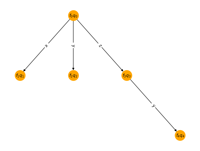
TernaryTree#
If you’ve built your own encoding, for instance using the TernaryTree class, you can also use this.
from ferrmion.visualise import draw_tt

tree = fr.TernaryTree(n_modes=5)
tree.add_node("zy")
tree.add_node("x")
tree.add_node("y")
tree.enumeration_scheme = tree.default_enumeration_scheme()
tree.build_encoding()
draw_tt(tree, type="standard", enumeration_scheme=tree.enumeration_scheme)
tree.encode(fham)
QubitHamiltonian({'IIIII': 18.9076311490779+0i, 'IIIIX': 0-0.054044855267008036i, 'IIIIY': 1.5570252447720878+0i, 'IIIIZ': -1.904902251450257+0i, 'IIIZI': 0.0673032609026337+0i, 'IIIZX': 0+0.05404485526700803i, 'IIIZY': -1.5570252447720878+0i, 'IIIZZ': -1.8455210285622243+0i, 'IIXII': 0+0.09194528485148387i, 'IIXIX': -0.09372480058823673+0i, 'IIXIY': 0-0.09956322292280037i, 'IIXIZ': 0-0.06398062582554465i, 'IIXZX': -0.006584524084405144+0i, 'IIXZY': 0+0.049921846765950344i, 'IIXZZ': 0+0.028231230883319566i, 'IIYII': 1.1994994625822795+0i, 'IIYIX': 0+0.1261284629092859i, 'IIYIY': -0.09925610140318297+0i, 'IIYIZ': -0.08678963265897728+0i, 'IIYZX': 0-0.07648708675243585i, 'IIYZY': -0.0010532232694588708+0i, 'IIYZZ': -0.04923414895740931+0i, 'IIZII': -1.68467299764772+0i, 'IIZIX': 0+0.19156313631216412i, 'IIZIY': -0.010695135161692848+0i, 'IIZIZ': 0.12094142501269206+0i, 'IIZZX': 0-0.19156313631216412i, 'IIZZY': 0.010695135161692848+0i, 'IIZZZ': -0.15210632381365122+0i, 'IXIII': 1.4711723106655499+0i, 'IXIIX': 0+0.11483104614317448i, 'IXIIY': -0.08139498712268023+0i, 'IXIIZ': 0.00006576012327344505+0i, 'IXIZX': 0-0.1156359828044034i, 'IXIZY': 0.07219065566469819+0i, 'IXIZZ': -0.06045787993999069+0i, 'IXXII': 0+0.14753041107216724i, 'IXYII': 0.0785806254379065+0i, 'IXZII': -0.047969782988100604+0i, 'IYIII': 0+0.034269571238060716i, 'IYIIX': -0.046409859644441845+0i, 'IYIIY': 0+0.00658192394259384i, 'IYIIZ': 0-0.006233734843999736i, 'IYIZX': 0.055614191102423896+0i, 'IYIZY': 0-0.007386860603822737i, 'IYIZZ': 0+0.15167760447941508i, 'IYXII': -0.0785806254379065+0i, 'IYYII': 0+0.14753041107216724i, 'IYZII': 0+0.029077434415576822i, 'IZIII': -2.0188019671438022+0i, 'IZIIX': 0-0.11771942960799285i, 'IZIIY': 0.036287664861934577+0i, 'IZIIZ': 0.13048181384245677+0i, 'IZIZX': 0+0.11771942960799285i, 'IZIZY': -0.036287664861934577+0i, 'IZIZZ': -0.08859828295605188+0i, 'IZXII': 0-0.14908376856335048i, 'IZYII': 0.03699300251288758+0i, 'IZZII': 0.23574710026205084+0i, 'XIIXI': 0.06284428800744621+0i, 'XIIYX': 0.0028929733946117947+0i, 'XIIYY': 0-0.000371862414990376i, 'XIIYZ': 0-0.0056239564519726115i, 'XIXXI': 0+0.11979992248556484i, 'XIXXX': -0.2608224533564394+0i, 'XIXXY': 0+0.10604779756515971i, 'XIXXZ': 0+0.06343039093935693i, 'XIXYI': -0.0023960952626263035+0i, 'XIXYX': 0-0.0014603929204522192i, 'XIXYY': -1.542674519425301+0i, 'XIXYZ': -1.8448827340725749+0i, 'XIYXI': 1.8448827340725749+0i, 'XIYXX': 0-0.10604779756515971i, 'XIYXY': -0.2608224533564394+0i, 'XIYXZ': 0.0023960952626263035+0i, 'XIYYI': 0+0.06343039093935693i, 'XIYYX': 1.5426745194253009+0i, 'XIYYY': 0-0.0014603929204522331i, 'XIYYZ': 0+0.11979992248556479i, 'XIZXI': 1.9185776348309769+0i, 'XIZXX': 0-0.11200173928332946i, 'XIZXY': -0.028728638861985636+0i, 'XIZXZ': -0.052942896570146475+0i, 'XIZYI': 0-0.06155836006233255i, 'XIZYX': 0.9821509553048453+0i, 'XIZYY': 0-0.1852474642087414i, 'XIZYZ': 0+0.2886439877855828i, 'XXXXI': 0-0.0013451335457962538i, 'XXXYX': 0+0.1147865789519015i, 'XXXYY': 0.09669961196484247+0i, 'XXXYZ': 0.017578033928802375+0i, 'XXYXI': 0.029910858777380596+0i, 'XXYYX': 0.06381908499534518+0i, 'XXYYY': 0+0.07255835656804532i, 'XXYYZ': 0+0.07621033422571782i, 'XXZXI': 0.10890704797913282+0i, 'XXZYX': -0.013534287040473186+0i, 'XXZYY': 0+0.047632417724760207i, 'XXZYZ': 0-0.12409578016633006i, 'XYXXI': -0.20180847815216735+0i, 'XYXYX': -0.0743562581682904+0i, 'XYXYY': 0-0.06824766115154023i, 'XYXYZ': 0-0.026941749471265278i, 'XYYXI': 0-0.050613718300248814i, 'XYYYX': 0+0.11047588353539639i, 'XYYYY': 0.08616243879189722+0i, 'XYYYZ': -0.15431958544598434+0i, 'XYZXI': 0+0.12409578016633006i, 'XYZYX': 0-0.047632417724760207i, 'XYZYY': -0.013534287040473186+0i, 'XYZYZ': 0.10890704797913282+0i, 'XZXXI': 0-0.27078507170064003i, 'XZXYX': 0-0.01060990101616291i, 'XZXYY': -0.09638481832588006+0i, 'XZXYZ': 0.09951450710339771+0i, 'XZYXI': -0.09951450710339771+0i, 'XZYYX': 0.09638481832588006+0i, 'XZYYY': 0-0.01060990101616291i, 'XZYYZ': 0-0.27078507170064003i, 'XZZXI': -0.2322946066416891+0i, 'XZZYX': 0.21512383704203647+0i, 'XZZYY': 0+0.0565412987386498i, 'XZZYZ': 0+0.029093525733964468i, 'YIIXI': 0-0.029093525733964468i, 'YIIYX': 0-0.0565412987386498i, 'YIIYY': 0.21512383704203647+0i, 'YIIYZ': -0.2322946066416891+0i, 'YXIXI': 0-0.05083052297699031i, 'YXIXX': -0.016650803881969836+0i, 'YXIXY': 0+0.024813275586719835i, 'YXIXZ': 0+0.1503265878280932i, 'YXIYI': -0.011860886922600886+0i, 'YXIYX': 0-0.12203034124991721i, 'YXIYY': 1.6506869653492973+0i, 'YXIYZ': 1.3603993594331272+0i, 'YXXXI': 0.017578033928802375+0i, 'YXXYX': 0.09669961196484247+0i, 'YXXYY': 0-0.1147865789519015i, 'YXXYZ': 0+0.0013451335457962538i, 'YXYXI': 0+0.07621033422571782i, 'YXYYX': 0+0.07255835656804532i, 'YXYYY': -0.06381908499534518+0i, 'YXYYZ': -0.029910858777380596+0i, 'YXZXI': 0-0.1309089557676221i, 'YXZYX': 0+0.004000859283264102i, 'YXZYY': 0.1138254471881604+0i, 'YXZYZ': -0.03297255049414944+0i, 'YYIXI': -1.360399359433127+0i, 'YYIXX': 0-0.024813275586719835i, 'YYIXY': -0.016650803881969836+0i, 'YYIXZ': 0.011860886922600886+0i, 'YYIYI': 0+0.1503265878280932i, 'YYIYX': -1.6506869653492973+0i, 'YYIYY': 0-0.12203034124991721i, 'YYIYZ': 0-0.05083052297699031i, 'YYXXI': 0-0.026941749471265278i, 'YYXYX': 0-0.06824766115154023i, 'YYXYY': 0.0743562581682904+0i, 'YYXYZ': 0.20180847815216735+0i, 'YYYXI': -0.15431958544598434+0i, 'YYYYX': 0.08616243879189722+0i, 'YYYYY': 0-0.11047588353539639i, 'YYYYZ': 0+0.050613718300248814i, 'YYZXI': 0.03297255049414944+0i, 'YYZYX': -0.1138254471881604+0i, 'YYZYY': 0+0.004000859283264102i, 'YYZYZ': 0-0.1309089557676221i, 'YZIXI': 0-0.2886439877855828i, 'YZIXX': 0.028728638861985636+0i, 'YZIXY': 0-0.11200173928332946i, 'YZIXZ': 0+0.06155836006233255i, 'YZIYI': -0.052942896570146475+0i, 'YZIYX': 0+0.1852474642087414i, 'YZIYY': 0.9821509553048453+0i, 'YZIYZ': 1.9185776348309769+0i, 'YZXXI': -0.06423161271570207+0i, 'YZXYX': 0.0964500346445237+0i, 'YZXYY': 0+0.06285586618432534i, 'YZXYZ': 0+0.025195599696344426i, 'YZYXI': 0-0.025195599696344426i, 'YZYYX': 0-0.06285586618432534i, 'YZYYY': 0.0964500346445237+0i, 'YZYYZ': -0.06423161271570207+0i, 'YZZXI': 0+0.0056239564519726115i, 'YZZYX': 0+0.000371862414990376i, 'YZZYY': 0.0028929733946117947+0i, 'YZZYZ': 0.06284428800744621+0i, 'ZIXII': 0+0.14908376856335048i, 'ZIYII': -0.03699300251288758+0i, 'ZIZII': 0.17251072768185632+0i, 'ZXIII': 0.047969782988100604+0i, 'ZXXII': 0-0.07787606730090726i, 'ZXXIX': -0.01428142449600213+0i, 'ZXXIY': 0+0.14183929138880882i, 'ZXXIZ': 0+0.053815241763404714i, 'ZXXZX': -0.07143231291895069+0i, 'ZXXZY': 0-0.09618885942822944i, 'ZXXZZ': 0-0.09109713050673937i, 'ZXYII': -1.582247638867951+0i, 'ZXYIX': 0-0.09495336844411444i, 'ZXYIY': -0.003345975475951654+0i, 'ZXYIZ': 0.1717432403988048+0i, 'ZXYZX': 0+0.04930293648353505i, 'ZXYZY': -0.08236776193900117+0i, 'ZXYZZ': -0.18967756459337848+0i, 'ZXZII': -1.4711723106655497+0i, 'ZXZIX': 0-0.1156359828044034i, 'ZXZIY': 0.07219065566469819+0i, 'ZXZIZ': -0.00006576012327344505+0i, 'ZXZZX': 0+0.11483104614317448i, 'ZXZZY': -0.08139498712268023+0i, 'ZXZZZ': 0.06045787993999069+0i, 'ZYIII': 0-0.029077434415576822i, 'ZYXII': 1.582247638867951+0i, 'ZYXIX': 0+0.04930293648353505i, 'ZYXIY': -0.08236776193900117+0i, 'ZYXIZ': -0.1717432403988048+0i, 'ZYXZX': 0-0.09495336844411444i, 'ZYXZY': -0.003345975475951654+0i, 'ZYXZZ': 0.18967756459337848+0i, 'ZYYII': 0-0.07787606730090726i, 'ZYYIX': 0.07143231291895069+0i, 'ZYYIY': 0+0.09618885942822944i, 'ZYYIZ': 0+0.053815241763404714i, 'ZYYZX': 0.01428142449600213+0i, 'ZYYZY': 0-0.14183929138880882i, 'ZYYZZ': 0-0.09109713050673937i, 'ZYZII': 0-0.034269571238060716i, 'ZYZIX': 0.055614191102423896+0i, 'ZYZIY': 0-0.007386860603822737i, 'ZYZIZ': 0+0.006233734843999736i, 'ZYZZX': -0.046409859644441845+0i, 'ZYZZY': 0+0.00658192394259384i, 'ZYZZZ': 0-0.15167760447941508i, 'ZZIII': -0.11297254852969835+0i, 'ZZXII': 0-0.09194528485148387i, 'ZZXIX': -0.006584524084405144+0i, 'ZZXIY': 0+0.049921846765950344i, 'ZZXIZ': 0+0.06398062582554465i, 'ZZXZX': -0.09372480058823673+0i, 'ZZXZY': 0-0.09956322292280037i, 'ZZXZZ': 0-0.028231230883319566i, 'ZZYII': -1.1994994625822795+0i, 'ZZYIX': 0-0.07648708675243585i, 'ZZYIY': -0.0010532232694588708+0i, 'ZZYIZ': 0.08678963265897728+0i, 'ZZYZX': 0+0.1261284629092859i, 'ZZYZY': -0.09925610140318297+0i, 'ZZYZZ': 0.04923414895740931+0i, 'ZZZII': -1.72887707489718+0i, 'ZZZIX': 0+0.08955283111864738i, 'ZZZIY': -0.013420657293724284+0i, 'ZZZIZ': -0.27698557118510925+0i, 'ZZZZX': 0-0.08955283111864738i, 'ZZZZY': 0.013420657293724284+0i, 'ZZZZZ': 0.17882256940610555+0i})
qham_annealed = tree.encode_annealed(fham)
qham_annealed
QubitHamiltonian({'IIIII': 18.9076311490779+0i, 'IIIIX': 0-0.0014603929204522331i, 'IIIIY': 1.542674519425301+0i, 'IIIIZ': -1.68467299764772+0i, 'IIIZI': 0.12094142501269206+0i, 'IIIZX': 0+0.0014603929204522192i, 'IIIZY': -1.5426745194253009+0i, 'IIIZZ': -1.904902251450257+0i, 'IIXII': 0-0.034269571238060716i, 'IIXIX': 0.0743562581682904+0i, 'IIXIY': 0-0.11047588353539639i, 'IIXIZ': 0-0.029077434415576822i, 'IIXZX': 0.08616243879189722+0i, 'IIXZY': 0+0.06824766115154023i, 'IIXZZ': 0+0.006233734843999736i, 'IIYII': 1.4711723106655497+0i, 'IIYIX': 0+0.1147865789519015i, 'IIYIY': 0.06381908499534518+0i, 'IIYIZ': -0.047969782988100604+0i, 'IIYZX': 0-0.07255835656804532i, 'IIYZY': 0.09669961196484247+0i, 'IIYZZ': 0.00006576012327344505+0i, 'IIZII': -2.0188019671438022+0i, 'IIZIX': 0-0.01060990101616291i, 'IIZIY': 0.09638481832588006+0i, 'IIZIZ': 0.23574710026205084+0i, 'IIZZX': 0+0.01060990101616291i, 'IIZZY': -0.09638481832588006+0i, 'IIZZZ': 0.13048181384245677+0i, 'IXIII': 1.9185776348309769+0i, 'IXIIX': 0+0.07648708675243585i, 'IXIIY': -0.006584524084405144+0i, 'IXIIZ': 0.06284428800744621+0i, 'IXIZX': 0-0.049921846765950344i, 'IXIZY': 0.0010532232694588708+0i, 'IXIZZ': -0.052942896570146475+0i, 'IXXII': 0-0.12409578016633006i, 'IXYII': 0.10890704797913282+0i, 'IXZII': -0.2322946066416891+0i, 'IYIII': 0+0.2886439877855828i, 'IYIIX': 0.09925610140318297+0i, 'IYIIY': 0-0.09956322292280037i, 'IYIIZ': 0-0.0056239564519726115i, 'IYIZX': -0.09372480058823673+0i, 'IYIZY': 0+0.1261284629092859i, 'IYIZZ': 0-0.06155836006233255i, 'IYXII': -0.10890704797913282+0i, 'IYYII': 0-0.12409578016633006i, 'IYZII': 0+0.029093525733964468i, 'IZIII': -1.8455210285622243+0i, 'IZIIX': 0+0.10604779756515971i, 'IZIIY': -0.2608224533564394+0i, 'IZIIZ': -0.15210632381365122+0i, 'IZIZX': 0-0.10604779756515971i, 'IZIZY': 0.2608224533564394+0i, 'IZIZZ': 0.0673032609026337+0i, 'IZXII': 0-0.15167760447941508i, 'IZYII': -0.06045787993999069+0i, 'IZZII': -0.08859828295605188+0i, 'XIIXI': 0.21512383704203647+0i, 'XIIYX': 0.03699300251288758+0i, 'XIIYY': 0+0.14908376856335048i, 'XIIYZ': 0+0.0565412987386498i, 'XIXXI': 0+0.12203034124991721i, 'XIXXX': -0.1717432403988048+0i, 'XIXXY': 0+0.053815241763404714i, 'XIXXZ': 0-0.004000859283264102i, 'XIXYI': -0.1138254471881604+0i, 'XIXYX': 0-0.07787606730090726i, 'XIXYY': -1.582247638867951+0i, 'XIXYZ': -1.6506869653492973+0i, 'XIYXI': 1.6506869653492973+0i, 'XIYXX': 0-0.053815241763404714i, 'XIYXY': -0.1717432403988048+0i, 'XIYXZ': 0.1138254471881604+0i, 'XIYYI': 0-0.004000859283264102i, 'XIYYX': 1.582247638867951+0i, 'XIYYY': 0-0.07787606730090726i, 'XIYYZ': 0+0.12203034124991721i, 'XIZXI': 0.9821509553048453+0i, 'XIZXX': 0-0.06398062582554465i, 'XIZXY': -0.08678963265897728+0i, 'XIZXZ': 0.0028929733946117947+0i, 'XIZYI': 0-0.000371862414990376i, 'XIZYX': 1.1994994625822795+0i, 'XIZYY': 0-0.09194528485148387i, 'XIZYZ': 0-0.1852474642087414i, 'XXXXI': 0+0.00658192394259384i, 'XXXYX': 0+0.026941749471265278i, 'XXXYY': 0.15431958544598434+0i, 'XXXYZ': 0.046409859644441845+0i, 'XXYXI': 0.08139498712268023+0i, 'XXYYX': 0.017578033928802375+0i, 'XXYYY': 0+0.07621033422571782i, 'XXYYZ': 0+0.11483104614317448i, 'XXZXI': -0.013420657293724284+0i, 'XXZYX': -0.06423161271570207+0i, 'XXZYY': 0-0.025195599696344426i, 'XXZYZ': 0-0.08955283111864738i, 'XYXXI': -0.055614191102423896+0i, 'XYXYX': -0.20180847815216735+0i, 'XYXYY': 0-0.050613718300248814i, 'XYXYZ': 0+0.007386860603822737i, 'XYYXI': 0-0.1156359828044034i, 'XYYYX': 0+0.0013451335457962538i, 'XYYYY': -0.029910858777380596+0i, 'XYYYZ': 0.07219065566469819+0i, 'XYZXI': 0+0.08955283111864738i, 'XYZYX': 0+0.025195599696344426i, 'XYZYY': -0.06423161271570207+0i, 'XYZYZ': -0.013420657293724284+0i, 'XZXXI': 0-0.024813275586719835i, 'XZXYX': 0-0.09109713050673937i, 'XZXYY': -0.18967756459337848+0i, 'XZXYZ': -0.016650803881969836+0i, 'XZYXI': 0.016650803881969836+0i, 'XZYYX': 0.18967756459337848+0i, 'XZYYY': 0-0.09109713050673937i, 'XZYYZ': 0-0.024813275586719835i, 'XZZXI': -0.028728638861985636+0i, 'XZZYX': -0.04923414895740931+0i, 'XZZYY': 0-0.028231230883319566i, 'XZZYZ': 0+0.11200173928332946i, 'YIIXI': 0-0.11200173928332946i, 'YIIYX': 0+0.028231230883319566i, 'YIIYY': -0.04923414895740931+0i, 'YIIYZ': -0.028728638861985636+0i, 'YXIXI': 0-0.05404485526700803i, 'YXIXX': -0.0023960952626263035+0i, 'YXIXY': 0+0.06343039093935693i, 'YXIXZ': 0+0.19156313631216412i, 'YXIYI': -0.010695135161692848+0i, 'YXIYX': 0+0.11979992248556484i, 'YXIYY': 1.8448827340725749+0i, 'YXIYZ': 1.5570252447720878+0i, 'YXXXI': 0.046409859644441845+0i, 'YXXYX': 0.15431958544598434+0i, 'YXXYY': 0-0.026941749471265278i, 'YXXYZ': 0-0.00658192394259384i, 'YXYXI': 0+0.11483104614317448i, 'YXYYX': 0+0.07621033422571782i, 'YXYYY': -0.017578033928802375+0i, 'YXYYZ': -0.08139498712268023+0i, 'YXZXI': 0-0.11771942960799285i, 'YXZYX': 0-0.27078507170064003i, 'YXZYY': -0.09951450710339771+0i, 'YXZYZ': 0.036287664861934577+0i, 'YYIXI': -1.5570252447720878+0i, 'YYIXX': 0-0.06343039093935693i, 'YYIXY': -0.0023960952626263035+0i, 'YYIXZ': 0.010695135161692848+0i, 'YYIYI': 0+0.19156313631216412i, 'YYIYX': -1.8448827340725749+0i, 'YYIYY': 0+0.11979992248556479i, 'YYIYZ': 0-0.054044855267008036i, 'YYXXI': 0+0.007386860603822737i, 'YYXYX': 0-0.050613718300248814i, 'YYXYY': 0.20180847815216735+0i, 'YYXYZ': 0.055614191102423896+0i, 'YYYXI': 0.07219065566469819+0i, 'YYYYX': -0.029910858777380596+0i, 'YYYYY': 0-0.0013451335457962538i, 'YYYYZ': 0+0.1156359828044034i, 'YYZXI': -0.036287664861934577+0i, 'YYZYX': 0.09951450710339771+0i, 'YYZYY': 0-0.27078507170064003i, 'YYZYZ': 0-0.11771942960799285i, 'YZIXI': 0+0.1852474642087414i, 'YZIXX': 0.08678963265897728+0i, 'YZIXY': 0-0.06398062582554465i, 'YZIXZ': 0+0.000371862414990376i, 'YZIYI': 0.0028929733946117947+0i, 'YZIYX': 0+0.09194528485148387i, 'YZIYY': 1.1994994625822795+0i, 'YZIYZ': 0.9821509553048453+0i, 'YZXXI': -0.013534287040473186+0i, 'YZXYX': 0.0785806254379065+0i, 'YZXYY': 0-0.14753041107216724i, 'YZXYZ': 0+0.047632417724760207i, 'YZYXI': 0-0.047632417724760207i, 'YZYYX': 0+0.14753041107216724i, 'YZYYY': 0.0785806254379065+0i, 'YZYYZ': -0.013534287040473186+0i, 'YZZXI': 0-0.0565412987386498i, 'YZZYX': 0-0.14908376856335048i, 'YZZYY': 0.03699300251288758+0i, 'YZZYZ': 0.21512383704203647+0i, 'ZIXII': 0+0.15167760447941508i, 'ZIYII': 0.06045787993999069+0i, 'ZIZII': 0.17882256940610555+0i, 'ZXIII': 0.2322946066416891+0i, 'ZXXII': 0-0.05083052297699031i, 'ZXXIX': -0.08236776193900117+0i, 'ZXXIY': 0+0.09618885942822944i, 'ZXXIZ': 0-0.1309089557676221i, 'ZXXZX': 0.07143231291895069+0i, 'ZXXZY': 0-0.04930293648353505i, 'ZXXZZ': 0+0.1503265878280932i, 'ZXYII': -1.360399359433127+0i, 'ZXYIX': 0-0.14183929138880882i, 'ZXYIY': 0.003345975475951654+0i, 'ZXYIZ': 0.03297255049414944+0i, 'ZXYZX': 0+0.09495336844411444i, 'ZXYZY': -0.01428142449600213+0i, 'ZXYZZ': 0.011860886922600886+0i, 'ZXZII': -1.9185776348309769+0i, 'ZXZIX': 0-0.049921846765950344i, 'ZXZIY': 0.0010532232694588708+0i, 'ZXZIZ': -0.06284428800744621+0i, 'ZXZZX': 0+0.07648708675243585i, 'ZXZZY': -0.006584524084405144+0i, 'ZXZZZ': 0.052942896570146475+0i, 'ZYIII': 0-0.029093525733964468i, 'ZYXII': 1.3603993594331272+0i, 'ZYXIX': 0+0.09495336844411444i, 'ZYXIY': -0.01428142449600213+0i, 'ZYXIZ': -0.03297255049414944+0i, 'ZYXZX': 0-0.14183929138880882i, 'ZYXZY': 0.003345975475951654+0i, 'ZYXZZ': -0.011860886922600886+0i, 'ZYYII': 0-0.05083052297699031i, 'ZYYIX': -0.07143231291895069+0i, 'ZYYIY': 0+0.04930293648353505i, 'ZYYIZ': 0-0.1309089557676221i, 'ZYYZX': 0.08236776193900117+0i, 'ZYYZY': 0-0.09618885942822944i, 'ZYYZZ': 0+0.1503265878280932i, 'ZYZII': 0-0.2886439877855828i, 'ZYZIX': -0.09372480058823673+0i, 'ZYZIY': 0+0.1261284629092859i, 'ZYZIZ': 0+0.0056239564519726115i, 'ZYZZX': 0.09925610140318297+0i, 'ZYZZY': 0-0.09956322292280037i, 'ZYZZZ': 0+0.06155836006233255i, 'ZZIII': 0.17251072768185632+0i, 'ZZXII': 0+0.034269571238060716i, 'ZZXIX': 0.08616243879189722+0i, 'ZZXIY': 0+0.06824766115154023i, 'ZZXIZ': 0+0.029077434415576822i, 'ZZXZX': 0.0743562581682904+0i, 'ZZXZY': 0-0.11047588353539639i, 'ZZXZZ': 0-0.006233734843999736i, 'ZZYII': -1.4711723106655499+0i, 'ZZYIX': 0-0.07255835656804532i, 'ZZYIY': 0.09669961196484247+0i, 'ZZYIZ': 0.047969782988100604+0i, 'ZZYZX': 0+0.1147865789519015i, 'ZZYZY': 0.06381908499534518+0i, 'ZZYZZ': -0.00006576012327344505+0i, 'ZZZII': -1.72887707489718+0i, 'ZZZIX': 0+0.06285586618432534i, 'ZZZIY': 0.0964500346445237+0i, 'ZZZIZ': -0.11297254852969835+0i, 'ZZZZX': 0-0.06285586618432534i, 'ZZZZY': -0.0964500346445237+0i, 'ZZZZZ': -0.27698557118510925+0i})
qham_topphatt = tree.encode_naive(fham)
qham_topphatt
QubitHamiltonian({'IIIII': 18.9076311490779+0i, 'IIIIX': 0-0.0014603929204522331i, 'IIIIY': 1.542674519425301+0i, 'IIIIZ': -1.68467299764772+0i, 'IIIZI': 0.12094142501269206+0i, 'IIIZX': 0+0.0014603929204522192i, 'IIIZY': -1.5426745194253009+0i, 'IIIZZ': -1.904902251450257+0i, 'IIXII': 0-0.034269571238060716i, 'IIXIX': 0.0743562581682904+0i, 'IIXIY': 0-0.11047588353539639i, 'IIXIZ': 0-0.029077434415576822i, 'IIXZX': 0.08616243879189722+0i, 'IIXZY': 0+0.06824766115154023i, 'IIXZZ': 0+0.006233734843999736i, 'IIYII': 1.4711723106655497+0i, 'IIYIX': 0+0.1147865789519015i, 'IIYIY': 0.06381908499534518+0i, 'IIYIZ': -0.047969782988100604+0i, 'IIYZX': 0-0.07255835656804532i, 'IIYZY': 0.09669961196484247+0i, 'IIYZZ': 0.00006576012327344505+0i, 'IIZII': -2.0188019671438022+0i, 'IIZIX': 0-0.01060990101616291i, 'IIZIY': 0.09638481832588006+0i, 'IIZIZ': 0.23574710026205084+0i, 'IIZZX': 0+0.01060990101616291i, 'IIZZY': -0.09638481832588006+0i, 'IIZZZ': 0.13048181384245677+0i, 'IXIII': 1.9185776348309769+0i, 'IXIIX': 0+0.07648708675243585i, 'IXIIY': -0.006584524084405144+0i, 'IXIIZ': 0.06284428800744621+0i, 'IXIZX': 0-0.049921846765950344i, 'IXIZY': 0.0010532232694588708+0i, 'IXIZZ': -0.052942896570146475+0i, 'IXXII': 0-0.12409578016633006i, 'IXYII': 0.10890704797913282+0i, 'IXZII': -0.2322946066416891+0i, 'IYIII': 0+0.2886439877855828i, 'IYIIX': 0.09925610140318297+0i, 'IYIIY': 0-0.09956322292280037i, 'IYIIZ': 0-0.0056239564519726115i, 'IYIZX': -0.09372480058823673+0i, 'IYIZY': 0+0.1261284629092859i, 'IYIZZ': 0-0.06155836006233255i, 'IYXII': -0.10890704797913282+0i, 'IYYII': 0-0.12409578016633006i, 'IYZII': 0+0.029093525733964468i, 'IZIII': -1.8455210285622243+0i, 'IZIIX': 0+0.10604779756515971i, 'IZIIY': -0.2608224533564394+0i, 'IZIIZ': -0.15210632381365122+0i, 'IZIZX': 0-0.10604779756515971i, 'IZIZY': 0.2608224533564394+0i, 'IZIZZ': 0.0673032609026337+0i, 'IZXII': 0-0.15167760447941508i, 'IZYII': -0.06045787993999069+0i, 'IZZII': -0.08859828295605188+0i, 'XIIXI': 0.21512383704203647+0i, 'XIIYX': 0.03699300251288758+0i, 'XIIYY': 0+0.14908376856335048i, 'XIIYZ': 0+0.0565412987386498i, 'XIXXI': 0+0.12203034124991721i, 'XIXXX': -0.1717432403988048+0i, 'XIXXY': 0+0.053815241763404714i, 'XIXXZ': 0-0.004000859283264102i, 'XIXYI': -0.1138254471881604+0i, 'XIXYX': 0-0.07787606730090726i, 'XIXYY': -1.582247638867951+0i, 'XIXYZ': -1.6506869653492973+0i, 'XIYXI': 1.6506869653492973+0i, 'XIYXX': 0-0.053815241763404714i, 'XIYXY': -0.1717432403988048+0i, 'XIYXZ': 0.1138254471881604+0i, 'XIYYI': 0-0.004000859283264102i, 'XIYYX': 1.582247638867951+0i, 'XIYYY': 0-0.07787606730090726i, 'XIYYZ': 0+0.12203034124991721i, 'XIZXI': 0.9821509553048453+0i, 'XIZXX': 0-0.06398062582554465i, 'XIZXY': -0.08678963265897728+0i, 'XIZXZ': 0.0028929733946117947+0i, 'XIZYI': 0-0.000371862414990376i, 'XIZYX': 1.1994994625822795+0i, 'XIZYY': 0-0.09194528485148387i, 'XIZYZ': 0-0.1852474642087414i, 'XXXXI': 0+0.00658192394259384i, 'XXXYX': 0+0.026941749471265278i, 'XXXYY': 0.15431958544598434+0i, 'XXXYZ': 0.046409859644441845+0i, 'XXYXI': 0.08139498712268023+0i, 'XXYYX': 0.017578033928802375+0i, 'XXYYY': 0+0.07621033422571782i, 'XXYYZ': 0+0.11483104614317448i, 'XXZXI': -0.013420657293724284+0i, 'XXZYX': -0.06423161271570207+0i, 'XXZYY': 0-0.025195599696344426i, 'XXZYZ': 0-0.08955283111864738i, 'XYXXI': -0.055614191102423896+0i, 'XYXYX': -0.20180847815216735+0i, 'XYXYY': 0-0.050613718300248814i, 'XYXYZ': 0+0.007386860603822737i, 'XYYXI': 0-0.1156359828044034i, 'XYYYX': 0+0.0013451335457962538i, 'XYYYY': -0.029910858777380596+0i, 'XYYYZ': 0.07219065566469819+0i, 'XYZXI': 0+0.08955283111864738i, 'XYZYX': 0+0.025195599696344426i, 'XYZYY': -0.06423161271570207+0i, 'XYZYZ': -0.013420657293724284+0i, 'XZXXI': 0-0.024813275586719835i, 'XZXYX': 0-0.09109713050673937i, 'XZXYY': -0.18967756459337848+0i, 'XZXYZ': -0.016650803881969836+0i, 'XZYXI': 0.016650803881969836+0i, 'XZYYX': 0.18967756459337848+0i, 'XZYYY': 0-0.09109713050673937i, 'XZYYZ': 0-0.024813275586719835i, 'XZZXI': -0.028728638861985636+0i, 'XZZYX': -0.04923414895740931+0i, 'XZZYY': 0-0.028231230883319566i, 'XZZYZ': 0+0.11200173928332946i, 'YIIXI': 0-0.11200173928332946i, 'YIIYX': 0+0.028231230883319566i, 'YIIYY': -0.04923414895740931+0i, 'YIIYZ': -0.028728638861985636+0i, 'YXIXI': 0-0.05404485526700803i, 'YXIXX': -0.0023960952626263035+0i, 'YXIXY': 0+0.06343039093935693i, 'YXIXZ': 0+0.19156313631216412i, 'YXIYI': -0.010695135161692848+0i, 'YXIYX': 0+0.11979992248556484i, 'YXIYY': 1.8448827340725749+0i, 'YXIYZ': 1.5570252447720878+0i, 'YXXXI': 0.046409859644441845+0i, 'YXXYX': 0.15431958544598434+0i, 'YXXYY': 0-0.026941749471265278i, 'YXXYZ': 0-0.00658192394259384i, 'YXYXI': 0+0.11483104614317448i, 'YXYYX': 0+0.07621033422571782i, 'YXYYY': -0.017578033928802375+0i, 'YXYYZ': -0.08139498712268023+0i, 'YXZXI': 0-0.11771942960799285i, 'YXZYX': 0-0.27078507170064003i, 'YXZYY': -0.09951450710339771+0i, 'YXZYZ': 0.036287664861934577+0i, 'YYIXI': -1.5570252447720878+0i, 'YYIXX': 0-0.06343039093935693i, 'YYIXY': -0.0023960952626263035+0i, 'YYIXZ': 0.010695135161692848+0i, 'YYIYI': 0+0.19156313631216412i, 'YYIYX': -1.8448827340725749+0i, 'YYIYY': 0+0.11979992248556479i, 'YYIYZ': 0-0.054044855267008036i, 'YYXXI': 0+0.007386860603822737i, 'YYXYX': 0-0.050613718300248814i, 'YYXYY': 0.20180847815216735+0i, 'YYXYZ': 0.055614191102423896+0i, 'YYYXI': 0.07219065566469819+0i, 'YYYYX': -0.029910858777380596+0i, 'YYYYY': 0-0.0013451335457962538i, 'YYYYZ': 0+0.1156359828044034i, 'YYZXI': -0.036287664861934577+0i, 'YYZYX': 0.09951450710339771+0i, 'YYZYY': 0-0.27078507170064003i, 'YYZYZ': 0-0.11771942960799285i, 'YZIXI': 0+0.1852474642087414i, 'YZIXX': 0.08678963265897728+0i, 'YZIXY': 0-0.06398062582554465i, 'YZIXZ': 0+0.000371862414990376i, 'YZIYI': 0.0028929733946117947+0i, 'YZIYX': 0+0.09194528485148387i, 'YZIYY': 1.1994994625822795+0i, 'YZIYZ': 0.9821509553048453+0i, 'YZXXI': -0.013534287040473186+0i, 'YZXYX': 0.0785806254379065+0i, 'YZXYY': 0-0.14753041107216724i, 'YZXYZ': 0+0.047632417724760207i, 'YZYXI': 0-0.047632417724760207i, 'YZYYX': 0+0.14753041107216724i, 'YZYYY': 0.0785806254379065+0i, 'YZYYZ': -0.013534287040473186+0i, 'YZZXI': 0-0.0565412987386498i, 'YZZYX': 0-0.14908376856335048i, 'YZZYY': 0.03699300251288758+0i, 'YZZYZ': 0.21512383704203647+0i, 'ZIXII': 0+0.15167760447941508i, 'ZIYII': 0.06045787993999069+0i, 'ZIZII': 0.17882256940610555+0i, 'ZXIII': 0.2322946066416891+0i, 'ZXXII': 0-0.05083052297699031i, 'ZXXIX': -0.08236776193900117+0i, 'ZXXIY': 0+0.09618885942822944i, 'ZXXIZ': 0-0.1309089557676221i, 'ZXXZX': 0.07143231291895069+0i, 'ZXXZY': 0-0.04930293648353505i, 'ZXXZZ': 0+0.1503265878280932i, 'ZXYII': -1.360399359433127+0i, 'ZXYIX': 0-0.14183929138880882i, 'ZXYIY': 0.003345975475951654+0i, 'ZXYIZ': 0.03297255049414944+0i, 'ZXYZX': 0+0.09495336844411444i, 'ZXYZY': -0.01428142449600213+0i, 'ZXYZZ': 0.011860886922600886+0i, 'ZXZII': -1.9185776348309769+0i, 'ZXZIX': 0-0.049921846765950344i, 'ZXZIY': 0.0010532232694588708+0i, 'ZXZIZ': -0.06284428800744621+0i, 'ZXZZX': 0+0.07648708675243585i, 'ZXZZY': -0.006584524084405144+0i, 'ZXZZZ': 0.052942896570146475+0i, 'ZYIII': 0-0.029093525733964468i, 'ZYXII': 1.3603993594331272+0i, 'ZYXIX': 0+0.09495336844411444i, 'ZYXIY': -0.01428142449600213+0i, 'ZYXIZ': -0.03297255049414944+0i, 'ZYXZX': 0-0.14183929138880882i, 'ZYXZY': 0.003345975475951654+0i, 'ZYXZZ': -0.011860886922600886+0i, 'ZYYII': 0-0.05083052297699031i, 'ZYYIX': -0.07143231291895069+0i, 'ZYYIY': 0+0.04930293648353505i, 'ZYYIZ': 0-0.1309089557676221i, 'ZYYZX': 0.08236776193900117+0i, 'ZYYZY': 0-0.09618885942822944i, 'ZYYZZ': 0+0.1503265878280932i, 'ZYZII': 0-0.2886439877855828i, 'ZYZIX': -0.09372480058823673+0i, 'ZYZIY': 0+0.1261284629092859i, 'ZYZIZ': 0+0.0056239564519726115i, 'ZYZZX': 0.09925610140318297+0i, 'ZYZZY': 0-0.09956322292280037i, 'ZYZZZ': 0+0.06155836006233255i, 'ZZIII': 0.17251072768185632+0i, 'ZZXII': 0+0.034269571238060716i, 'ZZXIX': 0.08616243879189722+0i, 'ZZXIY': 0+0.06824766115154023i, 'ZZXIZ': 0+0.029077434415576822i, 'ZZXZX': 0.0743562581682904+0i, 'ZZXZY': 0-0.11047588353539639i, 'ZZXZZ': 0-0.006233734843999736i, 'ZZYII': -1.4711723106655499+0i, 'ZZYIX': 0-0.07255835656804532i, 'ZZYIY': 0.09669961196484247+0i, 'ZZYIZ': 0.047969782988100604+0i, 'ZZYZX': 0+0.1147865789519015i, 'ZZYZY': 0.06381908499534518+0i, 'ZZYZZ': -0.00006576012327344505+0i, 'ZZZII': -1.72887707489718+0i, 'ZZZIX': 0+0.06285586618432534i, 'ZZZIY': 0.0964500346445237+0i, 'ZZZIZ': -0.11297254852969835+0i, 'ZZZZX': 0-0.06285586618432534i, 'ZZZZY': -0.0964500346445237+0i, 'ZZZZZ': -0.27698557118510925+0i})
Saved Encodings#
It’s possible to save an encoding, and re-use it later.
Let’s save and re-use the annealed encoding above.
import json
from ferrmion import MajoranaEncoding

annealed_qham= tree.encode_annealed(fham)

with open("data/saved_encoding.json", "w+") as f:
    json.dump(tree._encoding.to_json(), f)


with open("data/saved_encoding.json", "r") as f:
    data=json.load(f)

encoding = MajoranaEncoding.from_json(data)
qham_from_save = encoding.encode(fham)

assert qham_from_save == annealed_qham
Inbuilt Hamiltonians#
Molecular Hamiltonian#
This section shows how to use a Fermion-Qubit encoding to encode a second quantised Molecular hamiltonian.
Let’s first get the coefficients for our second quantised hamiltonian.
For the time being we can use randomly generated ones.
import ferrmion as fr
import numpy as np

constant_energy = 0
one_e_coeffs = np.random.random((3, 3))
two_e_coeffs = np.random.random((3, 3, 3, 3))
fermion_hamiltonian = fr.molecular_hamiltonian(
    one_e_coeffs=one_e_coeffs,
    two_e_coeffs=two_e_coeffs,
    constant_energy=constant_energy,
)
fermion_hamiltonian
FermionHamiltonian(+-, ++--, 3 modes, constant 0)
Hubbard Hamiltonian#
This notebook shows how to use a Fermion-Qubit encoding to encode the second quantised Hubbard hamiltonian.
The Hubbard Hamiltonian needs two scaler coefficients, the kinetic term \(t\) and the onsite-term \(U\).
We can either define both \(t\) and \(U\), or use the default \(t=1\) and scale \(U\) around it.
onsite_term = 2.0
hopping_term = 0.5
We can now make a Hamiltonian for the size of system we want to look at, let’s say 12 sites.
n_sites = 6
from ferrmion.hamiltonians import linear_adjacency_matrix

hamiltonian = fr.hubbard_hamiltonian(
    adjacency_matrix=linear_adjacency_matrix(n_sites, periodic=False),
    onsite_term=onsite_term,
    hopping_term=hopping_term,
)
hamiltonian
FermionHamiltonian(+-, +-+-, 6 modes, constant 0)
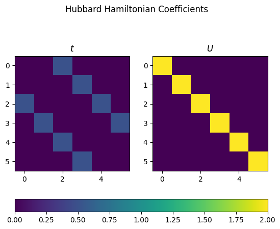
The function above will create matrices of coefficients for the “+-” and “+-+-” terms.
We can plot these to get a better idea of what they look like.
import matplotlib.pyplot as plt
from matplotlib import colors
import numpy as np

fig, axs = plt.subplots(1, 2)
fig.suptitle("Hubbard Hamiltonian Coefficients")
# create a single norm to be shared across all images
norm = colors.Normalize(vmin=np.min(0), vmax=np.max([onsite_term, hopping_term]))

axs[0].set_title("$t$")
axs[1].set_title("$U$")
images = []
images.append(axs[0].imshow(hamiltonian.terms["+-"], norm=norm))
# We use einsum to see the values for number operators
images.append(
    axs[1].imshow(np.einsum("iijj->ij", hamiltonian.terms["+-+-"]), norm=norm)
)
fig.colorbar(images[0], ax=axs, orientation="horizontal", fraction=0.1)
plt.show()
Finally, we can encode the Hamiltonian as before.
fr.Parity(hamiltonian.n_modes).encode(hamiltonian)
QubitHamiltonian({'IIIIII': 6+0i, 'IIIIIZ': -1+0i, 'IIIIXI': 0.25+0i, 'IIIIZZ': -1+0i, 'IIIXII': 0.25+0i, 'IIIZXZ': -0.25+0i, 'IIIZZI': -1+0i, 'IIYXXY': -0.25+0i, 'IIZXZI': -0.25+0i, 'IIZZII': -1+0i, 'IXIIII': 0.25+0i, 'IZXXXX': -0.25+0i, 'IZZIII': -1+0i, 'ZXZIII': -0.25+0i, 'ZZIIII': -1+0i})