Reduced Entanglement Ternary Tree

This notebook shows how to generate a reduced-entanglement ternary tree, with a method similar to that of 10.1103/PRXQuantum.5.030333

The MI matrix used later was derived by a different method than the p-GUCCSD in the original paper, namely from a tensor network.

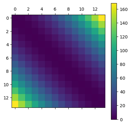
We’ll start with a full pairwise Mutual Information matrix for the 7 spatial orbitals of water in sto-3g.

import numpy as np

water_mi = np.array(
    [
        [0.0, 0.11687544, 0.07579407, 0.54274231, 0.59965614, 0.13984087, 0.1208934],
        [0.11687544, 0.0, -0.27575379, 0.44636705, 0.49251647, 0.04925079, 0.06179358],
        [0.07579407, -0.27575379, 0.0, 0.39213452, 0.64683832, 0.03424038, 0.4157573],
        [0.54274231, 0.44636705, 0.39213452, 0.0, 0.8947678, 0.47164455, 0.44469482],
        [0.59965614, 0.49251647, 0.64683832, 0.8947678, 0.0, 0.49754887, 0.48494587],
        [0.13984087, 0.04925079, 0.03424038, 0.47164455, 0.49754887, 0.0, 0.0067195],
        [0.1208934, 0.06179358, 0.4157573, 0.44469482, 0.48494587, 0.0067195, 0.0],
    ]
)

We can plot this to get a better understanding of what’s going on.

import matplotlib.pyplot as plt
import matplotlib.pyplot as plt

plt.matshow(water_mi)
plt.colorbar()

<matplotlib.colorbar.Colorbar at 0x10cc65550>

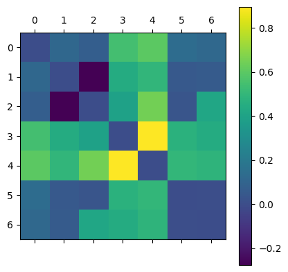
So it looks like spatial orbitals 3 and 4 generally have high mutual information with others. This is good (!) as these orbitals sit at the fermi-level.

In particular we see that spatial orbitals 3 and 4 are highly correlated with eachother, so to produce a reduced entanglement tree, we expect that spin orbitals \(3 \to (6,7)\) and \(4 \to (8,9)\) should be put in a parity (x) branch together.

Let’s create a rett, allowing only 1 X-branch.

from ferrmion.optimize.rett import reduced_entanglement_ternary_tree

rett = reduced_entanglement_ternary_tree(mutual_information=water_mi, max_branches=1)

To see what nodes exist, and what modes and qubit are mapped to them, we can check the tree’s enumeration scheme.

rett.enumeration_scheme

{'': (6, 6),
 'x': (7, 7),
 'xx': (8, 8),
 'xxx': (9, 9),
 'z': (0, 0),
 'zz': (1, 1),
 'zzz': (2, 2),
 'zzzz': (3, 3),
 'zzzzz': (4, 4),
 'zzzzzz': (5, 5),
 'zzzzzzz': (10, 10),
 'zzzzzzzz': (11, 11),
 'zzzzzzzzz': (12, 12),
 'zzzzzzzzzz': (13, 13)}

This actually show’s what we wanted, but it’s clearer with a visualisation.

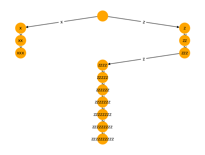
First let’s just see the structure of the tree…

from ferrmion.visualise import draw_tt

draw_tt(rett)

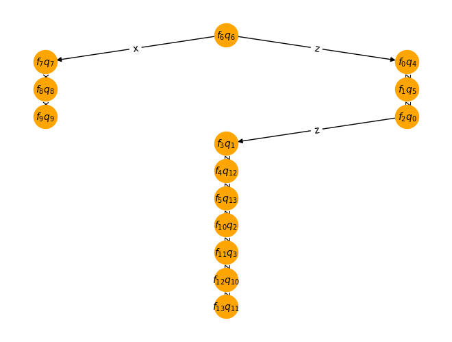
Finally, we label the tree drawing with the tree’s enumeration scheme.

draw_tt(rett, enumeration_scheme=rett.enumeration_scheme)

As expected, the spin-orbitals (fermionic modes) {6,7,8,9} now live on an X-branch together, with the other orbitals on a Z-branch.

We can additionaly use an evolutionary algorithm to optimize the enumeration scheme.

In the original paper, they minimise a cost function which weights the MI by the distance squared.

n_mode = rett.n_modes

distance_matrix = np.array(
    [[np.abs(i - j) ** 2 for j in range(n_mode)] for i in range(n_mode)]
)

plt.matshow(distance_matrix)
plt.colorbar()

<matplotlib.colorbar.Colorbar at 0x10cc5a850>

This cost function is available in ferrmion.optimize.

We need to provide the MI matrix, and a permutation of spatial orbital indices.

Note because we’re using a spinless MI matrix, we only need half the number of indices.

from ferrmion.optimize import distance_squared, minimise_mi_distance

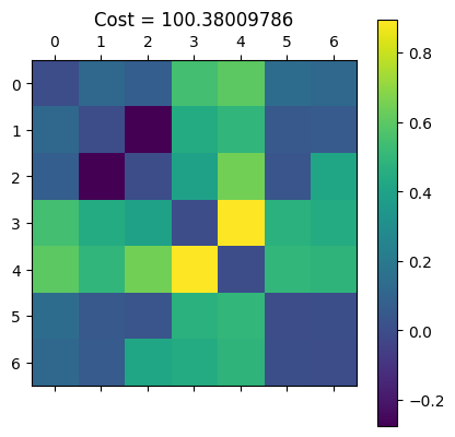
naive_permutation = [i for i in range(rett.n_modes // 2)]

distance_squared(water_mi, naive_permutation)

[np.float64(100.38009786)]

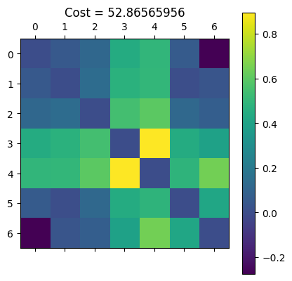
To find an approximately optimal permutation, we can use the lambda+mu evolutionary algorithm.

best_permutation = minimise_mi_distance(
    water_mi, pop_size=1000, ngen=50, pair_spins=False
)
print(best_permutation)

[2 6 4 3 0 5 1]

Now let’s compare the naive enumeration scheme to the optimized one:

plt.matshow(water_mi)
plt.title(f"Cost = {distance_squared(water_mi, naive_permutation)[0]}")
plt.colorbar()

plt.matshow(water_mi[best_permutation][:, best_permutation])
plt.title(f"Cost = {distance_squared(water_mi, best_permutation)[0]}")
plt.colorbar()

<matplotlib.colorbar.Colorbar at 0x10d36ccd0>

Create a map from the spatial orbital permutation to spin-orbitals

for each spatial orbital \(\Psi\), we need two spin orbitals \(\chi^\alpha\) and \(\chi^\beta\)

\[\Psi_i \to \set{\chi_{2i}^\alpha, \chi_{2i+1}^\beta}\]

# i -> (2i, 2i+1)
pos_map = {int(2 * best): 2 * i for i, best in enumerate(best_permutation)}
pos_map.update(
    {int(2 * best) + 1: 2 * i + 1 for i, best in enumerate(best_permutation)}
)
enumeration_scheme = {
    k: (v[0], pos_map[v[1]]) for k, v in rett.enumeration_scheme.items()
}

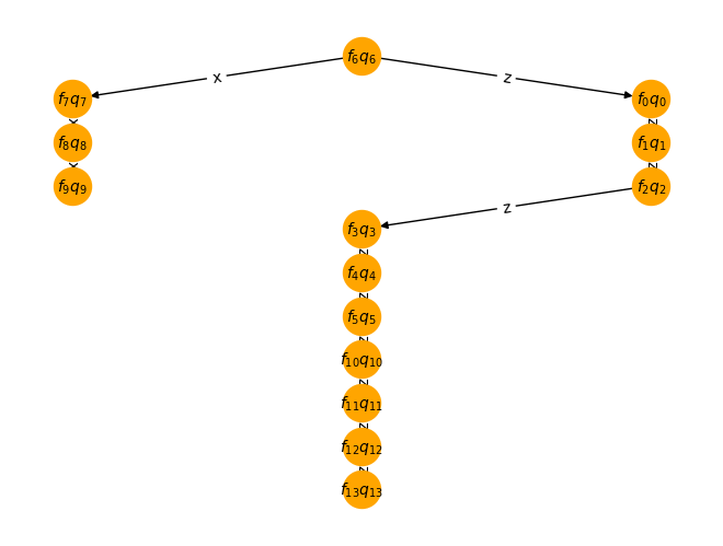
We can now redraw the tree with its new enumeration scheme.

rett.enumeration_scheme = enumeration_scheme
draw_tt(rett, enumeration_scheme=enumeration_scheme)